Spiral patterns in shells & horns
Where we use a mathematical approach to
model the shape of shells and horns of various kinds, with a special
emphasis on the Nautilus.
Modeling shell and horn geometry
In this section, we introduce the mathematical concepts needed to
model a great variety of seashells and horns.
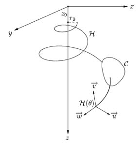
The logarithmic helico-spiral
|
Figure 3.1: Logarithmic helico-spiral and its "shadows".
|
|
As explained in the opening chapter, the pattern that shells exhibit
are governed by logarithmic spirals of various kinds. For the
Nautilus shell, the spiral lies in a plane P dividing the shell
into two symmetric pieces. But for most other shells, the growth takes
place along a logarithmic spiral which has been stretched along a
coiling axis going through the pole and normal to P, axis we
conveniently call the z-axis. This curve is the so-called
logarithmic helico-spiral, which we denote H, and has the
following parametric
representation in cylindrical coordinates:
| |
H= H(q) = |
ě
ď
í
ď
î
|
|
x(q) = r0 eqcota cosq= r(q) cosq |
|
|
y(q) = r0 eqcota sinq= r(q) sinq |
|
|
|
|
|
| | a, b Î |
ů
ű
|
0, |
p
2
|
é
ë
|
, r0, z0 Î R. |
| |
|
For physical reasons, we choose q Î ]0, qmax[, where q
= 0 at the apex of the shell, and q
= qmax at its opening.
In most shells, the angles a and b are equal, and thereby
H moves on a right cone and its pole O is at the cone's apex. In
fact, the angle j between the coiling axis and the line
(OP), where P is moving on H, is given by tanj = r(q) / z(q) = r0 / z0. As can be seen, this angle is
independent of q, and hence P will never leave the cone, whose
opening angle is arctan (r0 / z0). If a and
b are not equal, the proportion r(q) / z(q) depends on
q, so the spiral does not move along a straight cone. As a
consequence, the sought self-similarity properties are lost and
therefore, this shape is not very common among shells. So in the
following, it is assumed that a = b, i.e. that ř(q) = ž (q).
|
Generating curve and Frenet-Serret frame
|
When constructing the surface of a shell, we sweep a curve C along
H, having the shape of the shell's aperture. This curve is called
the generating curve and determines the profile of the shell.
For example, in common shells such as the snail, this curve is
approximately a half ellipse. However, more exotic variants have more
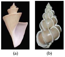
complicated generating curves, such as the Thatcheria
mirabilis shown on figure 3.3 (a).
|
Figure 3.3: Thatcheria mirabilis and Epitonium
scalare.
|
The generating curve is defined in a local coordinate system
uvw with origin moving along H. But there are various ways to
orientate the coordinate axes. For instance, most shells exhibit
orthoclinal growth, which means that the instantaneous
tangent of H is normal to C, assumed to lie in the plane uv
(cf. figure 3.4). This is particularly visible
in the Epitonium scalare (figure 3.3
(b)), where the white ribs are not vertical but perpendicular to the
spiral. Thus, it would be convenient to let the coordinate system
uvw alone determine the orientation of C, so that we do not have
to worry about this when defining C. In the orthoclinal growth
case (illustrated on figure 3.4), we orient
w along the unit tangent vector et of H. The vectors u and
v are aligned with the unit principal normal vector en and the
unit binormal vector eb of H, respectively. The triple {et,en, eb} is called the Frenet-Serret frame on H, and
the components are defined by the relations
|
et = |
H˘(q)
|| H˘(q) ||
|
, en = et ×eb, eb = |
H˘(q) ×H" (q)
|| H˘(q) ×H" (q) ||
|
, |
|
where || ·|| denotes the usual Euclidean norm in
R3. These formulas are well known in differential geometry,
so we will not prove them right here (proofs can be found in [8]) and
in [9]. One should note, however, that the
Frenet-Serret frame is defined provided that H and
H˘ are both regular. But this is
obviously the case here, since H" never vanishes.
Figure 3.4: Construction of the shell with orthoclinal growth.
When we are not dealing with orthoclinal growth, which is the
case when modeling the Nautilus, we do not need Frenet-Serret frames.
The coordinate system uvw is simply translated and rotated so that
its pole lies on H and that u and v are perpendicular and
parallel to the z-axis, respectively. We will call this kind of
growth vertical.
Now we need to scale C in order to get a surface whose
aperture grows exponentially, in accordance with the exponential
growth of the animal. Obviously, to preserve the self-similarity
properties, C and H must grow at the same rate, which we call
s. We put s = r(q) in order to express the growth rate
qualitatively. Proper constants will be added in Raup's Model which we
will encounter in the next section. So, the system uvw is defined,
in the vertical case, as
| |
|
| |
| |
|
| |
| |
|
| u(q) ×v(q) = s2 (sinq, cosq, 0) |
| |
|
In the orthoclinal case, we have, of course, (u(q), v(q), w(q)) = s ·(et, en, eb).
The mathematical aspects being clarified, we are ready to
bring the pieces together in Raup's Coiling Model.
The Raup Coiling Model
The physical model
In 1962, Raup, [21] and [22], introduced a model of
seashells consisting of four parameters whose meaning he expressed as
follows:
A simple model of variation in the rate of
growth in several dimensions accounts for variation in the form of
gastropod shells. The model specifies the shape of the aperture,
or generating curve, the axis of coiling, the size ratio (W) of
successive generating curves, the distance (D) of the generating
curve from the axis, and the proportion (T) of the height of one
generating curve that is covered by the successive
gyres.
This definition is very vague, but this has no importance; the
important thing is namely the meaning of the four parameters,
and the exact definition is up to us to formulate. In fact, when
studying the morphology of shells and horns, one can imagine that a
certain definition might be better suited for a special experimental
device than another. So here is our definitions of the
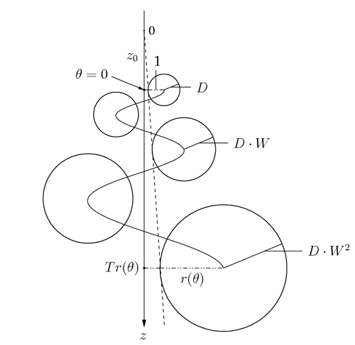
parameters W, D and T (illustrated on figure
3.5) 3:
- W is the factor by which C is magnified at each
revolution. So, for instance, if W = 2 and C is a circle, the
diameter of C is doubled after a revolution.
- D is the length, at q
= 0, from the center of C to the
orthogonal projection, onto the radius vector r0, of the closest
point on C to the z-axis. So, if again C is a circle, D
is the radius of C at q
= 0. It is not difficult to figure
out that, with this definition, we can indeed vary the distance from
C to the z-axis, since we thereby vary the slope of the inner
tangent to the shell's surface (dotted line on the figure).
- T is the ratio between z(q) and r(q).
Figure 3.5: Schematic section of a seashell with Raup's Coiling
Model parameters shown.
To get an intuitive feeling of the meaning of Raup's Coiling Model
parameters, try the Raup Coiling Model
applet, where you can modify these in real-time on a three
dimensional surface.
From a physical to a mathematical model
Our interpretation of Raup's model is well suited when we have
sections of seashells, such as the one schematized on figure
3.5. However, when constructing the shell, we are
interested in knowing the parameters needed in the mathematical model,
such as the angle a or the initial radius r0, only
implicitly contained in W, D and T. It is, however,
straightforward to convert these parameters, as we will show now.
Let us consider a shell which does not exhibit orthoclinal
growth, and whose generating curve C is a circle lying in the uv
plane. This is the most simple setup, and it does not affect the
following results when extended to more general cases. Now consider
the projection of H onto the xy-plane, which is the logarithmic
spiral given by the equation r = r0 eqcota (actually,
this spiral is a special case of a helico-spiral with z0 = 0 in the
parametrization ). The generating curve C
is thereby projected onto a straight line segment aligned with the
radius vector. Since the length of this segment is multiplied by W
at each revolution, we get immediately, by theorem
2.3.4, that a = arccot ( ln(W) / 2p). Furthermore, we have chosen r0 = 1 for
simplification, and this of course does not affect the model, since it
is only a matter of scaling. As a consequence, D, being the radius
of C at this point (q
= 0), will most often be chosen in the
interval ]0,1]. If D is chosen greater that 1, the generating
curve will be on both sides of the z-axis, yielding odd shells that
we have not encountered. T being the ratio between z(q) and
r(q), we have in particular that z(0) / r(0) = z0 / r0 = z0 = T, so it is throught z0 that the stretching parameter T is
expressed.
Shell generation
We are now ready to construct the seashell. So let
|
C= C(t) = (xC(t), yC(t), zC(t)) |
|
be a parametrization of C in uvw. Then the shell has the
parametrization
|
S= S(q, t) = H(q) + D ·C(t) ·(u(q), v(q), w(q))T. |
|
In a sketchy way, what happens here is that C is translated by the
vector H(q), and thereby its center lies on H (by center we
mean the origin of the coordinate system in which C is defined).
Then C is scaled and rotated properly by means of the uvw
system. Examples that illustrate the difference between the two growth
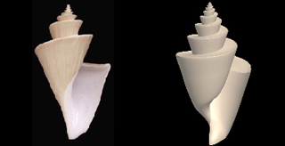
types are shown on figure 3.6.
Figure 3.6: Seashell models with vertical (left) and orthoclinal
(right) growth.
A more realistic generating curve
The above seashell models have been generated by a circle. However,
this is a very simplistic model which is not realistic. In fact, the
great diversity in shells is essentially provided by the different
kinds of generating curves. This is clearly illustrated in the
Thatcheria on figure 3.3. And there
are many ways to represent shapes that can not be approximated by
simple mathematical curves such as the circle. One of the ways is to
use Bézier curves, which provide a very simple and intuitive
representation of polynomial curves by means of control points. The
use of Bézier curves is, nevertheless, not in the scope of this
report. In fact, the problem is that, when using such curves, we move
away from the initial driving idea, that is, that nature is built up
around a few, simple and very precise elements. And the reason for
these elements being present instead of others is clear. But when the
generating curve is "arbitrary", and therefore best approximated
using polynomial curves, we can not answer this question,
"why?", anymore, and therefore it is of very limited
interest that we study them. However, it yields some very beautiful
pictures as well as interesting mathematical problems, and therefore
we have tried, using these curves, to model shells which, concerning
the generating curve, have no obvious reason to have the shape
it has instead of any other!
Making the attempt to model seashells using Bézier curves was
inspired by [7]. Other attemps have been made, for
instance by Michael Cortie, as described in [10]. The idea
is basically the same, except that Cortie includes parameters which
control rotations of the uvw coordinate system, and thus, he is not
limited to the vertical and orthoclinal cases - but they are more or
less the only ones present in nature.
The Raup Coiling Model applied to various shells
Most shells and horns are simple enough to be modeled using Raup's
Coiling Model, and in this section we apply it to construct several
surfaces. Special emphasis has been put in the modeling of Nautilus,
and other more or less comlicated figures are shown without further
descriptions. They are simply the result of different Raup model
parameter combinations and generating curves.
The Nautilus shell
The nautiloid family
|
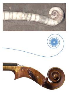
Figure 3.7: The lituus (middle) found in various shapes: (top) the
Lituite Lituus; (bottom) a violin neck.
|
The Nautilus pompidus (or simply Nautilus) is a
mollusc belonging to the family of Nautiloids, which itself
belongs to the wider family of marine molluscs called the
Cephalopods. They emerged in the late Cambrian,
approximately 500 million years ago, and are characterized by their
chambered shell, where the outermost chamber is the one where the
animal lives. The chambers are separated by walls (called
septa) with a small funnel (the siphuncle), allowing
the Nautiloid to inject a gas, essentially nitrogen, that will make it
float.
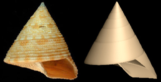
Many different molluscs descended from this family, and among
those, the Orthoceras, whose shell had a conical structure
(cf. figure 2.11). According to the (unknown) author
of the website [4], Most early
nautiloids had straight conical shells.. However,
these species did not survive; instead, new species developed by
coiling their shell. An example of an "intermediate" species is the
so-called Lituite Lituus, a "half-coiled up" cone (as shown
of figure 3.7 (top)). The shell follows a curve which
neither a straight line nor a logarithmic spiral, as in the two above
mentioned extremes, but a lituus (figure 3.7
(middle)), whose polar equation is r = a / Ö{q}. This curve is
also found extensively in architectural design, a known example being
the neck of a violin.
|
The Lituite Lituus did not survive either. In fact,
today there are only a few species left from the Nautiloid family (3
or 4, according to [14]) and they all belong to the
Nautilus genus. This suggests somewhat that the Nautilus had better
survival capabilities, which is quite understandable because of the
more compact, and thereby less fragile, shape of the shell, compared
to the conical or "semi-conical" ones of the Orthoceras and Lituite
Lituus, respectively. It is also an interesting fact to know that the
Nautilus migrates from depths of 500 meters to the water surface, by
regularizing the gas in its chambers. This indicates the strength of
its shell, tolerating extreme changes in pressure as well as
temperature.
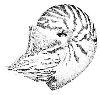 Figure 3.8: A swimming Nautilus (illustration taken from
http://waquarium.mic.hawaii.edu/MLP/root/html/MarineLife/Invertebrates/Molluscs/Nautilus.html).
Figure 3.8: A swimming Nautilus (illustration taken from
http://waquarium.mic.hawaii.edu/MLP/root/html/MarineLife/Invertebrates/Molluscs/Nautilus.html).
Measurements on the Nautilus shell
The spiral of the Nautilus lies in a plane, and Therefore, T = 0.
Furthermore, it seems reasonable to believe that the generating curve
is tangent to the coiling axis, and thereby that D = 1. We have
measured the constant by which the radius is incremented at each
revolution, and found that in average, W = 2.93. We are not in
possession of any precise measuring tool, so this result should not be
taken seriously! However, the measurements on each shell are almost
identical, which indicates that the actual Nautilus has found its very
precise shell shape. On the website www.spirasolaris.com, John
N. Harris points out that this growth constant is approximately equal
to f7/3 @ 3.07353, f being
the Golden Ratio that we will encounter in the next chapter. We do not
know if this is a coincidence, but believe that the relation is a bit
far-fetched, and has no interesting significance in our work.
Concerning the generating curve, it cannot be approximated by
a simple mathematical curve, although one could argue that an ellipse
does the job. We are not interested in that solution, especially
because the curve is three dimensional, as depicted on the profile
view of figure 3.9 (right). Therefore, to
be as realistic as possible, we use the Bézier curves. We would like
to emphasize on the fact that this choice is only made in order to
model a beautiful and an as-realistic-as-possible shell surface. But,
in the context of shapes generated by nature, we do not like the idea,
since there is no explanatory value in an arbitrary curve which Bézier
curves are. However, we can still suggest the reason for the apertures
actual shape.
To that purpose, let us, conceptually, build up the Nautilus
shell. As a starting point, we assume that the parameters W and T
are known. In fact, that T = 0 is obvious because of the upstanding
posture of the Nautilus. If T ą 0, the shell would not be
symmetric, and thereby the animal would not be in its natural
equilibrium position (cf. figure 3.8). The
growth rate may also be assumed known, since it has no mathematical
importance here, as long as it is greater than 1. Now imagine that the
aperture of the shell is a circle which is tangent to the underlying
whorl. Mathematically, this would be a perfect model expressing the
same kind of growth as the Nautilus', that is, along a logarithmic
spiral lying in a plane P. Such a "mathematical Nautilus" is
shown on figure 3.10 (a). Now let us analyse
a cross section of the shell generated by a plane perpendicular to
P going through the pole of the spiral (figure
3.10 (b)). Clearly, this setup is not very
well suited for several reasons: the innermost whorls of the shell are
exposed to the surrounding environment; the structure is unstable
because there is only one contact point between two neighboring whorl
circles. A much more robust setup would be to imbricate the whorls, as
depicted on figure 3.10 (c) and illustrated
with the Ammonite of figure 3.10
(d). But proceeding to the extreme, why not let one whorl cover all
the other ones? This is what we think the Nautilus has done when
developing from the primitve Orthoceras to its actual shape, but we
haven't got any confirmation of this. Another advantage of this
configuration is that it permits the animal inside to adhere better to
the shell because of the "bump" created by the underlying whorl
(instead of the convex surface that the circle would result in).
Figure 3.10: (a) A mathematical Nautilus; (b) cross-section
of (a); (c) an optimized (b); (d) a real Ammonite.
Of course, this "theory" in the shell's development can not
be proved in the way T. A. Cook, Moseley and others for instance
proved the presence a logrithmic spiral in shells. This is due to the
fact that we are now moving into domains of evolution which are more
complex, in the sense that a lot more factors govern the shape of the
aperture, and it is therefore not suitable for a deeper mathematical
study.
The model
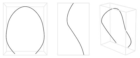
The curve C we have used to generate the surface is shown,
from different viewpoints, on figure 3.11.
Figure 3.11: The generating curve of the Nautilus from
different viewpoints: front, profile, combined.
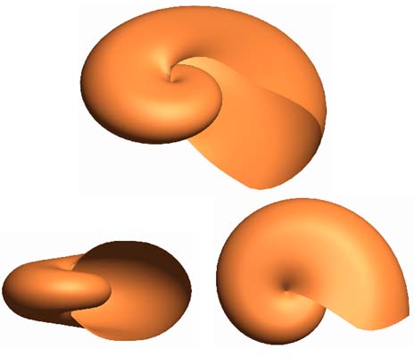
The result of coiling the Nautilus' generating curve around the
z-axis, with the parameters W = 3, D = 1 and T = 0 is shown on
figure 3.12.
Figure 3.12: The Nautilus shell model.
Other kinds of shells, horns
With the above described model, combining Frenet-Serret frames with
Raup's Coiling Model and Bézier curves, it is only a matter of will to
model any kind of shells. This section is meant as an illustration of
this purpose, without going into the details of each specific shell's
constructions. We shall only mention that, in some cases, the formula
for the seashell has been modified slightly in order to model bumps
and ribs, often present on the surfaces. This is actually
straightforward. Recall from section 3.1.3 that D is a
constant controlling the overall magnification of the C, in
particular its dimensions at q
= 0. By making it a function of
q, we can vary the magnification throughout a revolution, for
instance using the bell-shaped function e-pt2. An example of
such a shell is the Epitonium scalare, the second figure below.
|

|
|
Astele Armillatum
|
Epitonium Scalare
|

|
|
|
Ficus Filosa
|
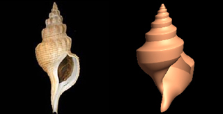
Penion Mandarinus
|
|
|
|
Thatcheria Mirabilis
|
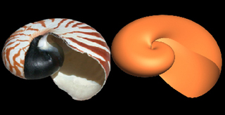
Nautilus Pompilus
|
|
|
|
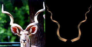
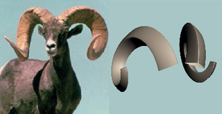
Greater Kudu
|
Wild sheep
|
Pictures of the models can be found in much greater resolution in
the 3D shell and horns gallery.
Discussion
Many attemps to model seashells using a computer have been made,
starting from David Raup in 1962. The following models have more or
less been based on this one, with some improvements. In particular,
Prusinkiewicz et al. [7] added, in 1992, textures to the shell
surface, while Cortie [10] made, in 1993, a 16 parameter model which
gave more freedom in the orientation of the uvw coordinate system and
integrated ribs and bumps explicitely in the formula for the shell. As
you may have noticed, these are all very recent works, indicating that
modeling of these relatively simple shapes found in nature still
reveal great challenge if one wishes to understand them
completely.
We shall end this chapter by showing an example of a shell
which cannot be modelled using our model or any of the above
mentioned. In fact, the lack of self-similarity (due to the sudden
change in the apertures shape) makes this, in the essence, impossible.
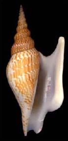 Figure 3.13: Strombus Listeri.