Two dimensional spirals

... also known as equiangular spirals, Bernoulli spirals, proportional spirals, geometrical spirals, spira mirabilis.

A brief history and definitions

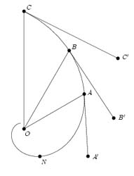
In a letter dated 12th of september 1638 and addressed to Mersenne, Descartes wrote: ... for this spiral, it has several properties which makes it quite recognizable. Because if O is the centre of the earth and that ONABC is the spiral, having traced straight lines OA, OB, OC and similar, there is the same proportion between the curve ONA and the line OA than between the curve ONAB and the line OB, or ONABC and OC, and so on for the remaining. Furthermore, if one traces the tangents AA˘, BB˘, CC˘ etc., the angles OAA˘, OBB˘, OCC˘ etc. will be equal.

This paragraph is considered as the one giving birth to the logarithmic spiral. It reveals its many mathematical aspects, and these have all yielded different names attributed to it. The fundamental property of the spiral is that the angle between an arbitrary tangent to the curve at a point P and the corresponding radius vector OP is constant. Therefore, René Descartes called it the equiangular spiral.

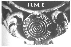
Figure 2.1: Photo of Bernoulli's tomb. Try to find the mistake made by the sculptor...

A few decenies later, namely in 1691 in Acta eruditorum, Jacob Bernoulli called it the logarithmic spiral because the vector angle about the pole is proportional to the logartihm of the corresponding radius. He eventually became so fascinated by this curve that he had it engraved on his tomb (cf. figure 2.1), followed by the phrase "Eadem mutata resurgo", meaning "I shall arise the same, though changed". Soon, the reader will understand the mysterious meaning of that phrase, and how it is related to this specific curve. He also called it spira mirabilis, which means "admirable spiral". He was truly amazed.

In Descartes' above description, it is mentioned that there are similarities in proportions, which in 1696 led Edmund Halley in Philosophical Transactions to call it the proportional spiral, noting that The lengths of segments cut off from a radius vector between successive whorls of the spiral form a geometric progression. The last most known name for the spiral is due to P. Nicolas, who called it the geometric spiral (De Novis Spiralibus, 1693), and was based on a similar observation to Halley's.

Long before the logarithmic spiral was discovered, Archimedes (287-212 BC) in On Spirals introduced another spiral, named after him: the Archimedean spiral. It is not to be mistaken for a logarithmic spiral. Indeed, most of the interesting properties of the logarithmic spiral, which we shall study in the following, are not present in an archimedean spiral.

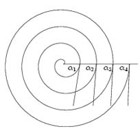
Figure 2.2: An archimedean spiral with a few of its tangents. Compare this shape with the one on the photo from the previous page.

The archimedean spiral is the trajectory of a point P moving uniformely away from a point O (the pole) and meanwhile rotating uniformly around this pole. Thus, there is a linear relation between the radius OP, denoted r, and the angle of rotation, q, and the archimedean spiral with pole at the origin of a polar coordinate system is therefore given by the equation r = aq, a being a characteristic constant of the spiral. So, using Halley's formulation, the lengths of segments cut off from a radius vector between successive whorls of the spiral are all equal. And it is exactly the fact that they are equal - hence do not progress - that distinguishes it from the logarithmic spiral, which we will see is the mathematical expression of growth. Furthermore, the angle a between a radius vector at a given point and the tangent to the curve at this point is given by the relation

tana =

r dq

= q,

which shows that a continuously tends to p/2 as q goes to infinity (cf. figure 2.2). This being said, we now turn our interest exclusively towards the logarithmic spirals.

The diversity in the names attributed to the curve reveals that we are dealing with a curve having many aspects. This is in particular visible in the various ways of defining the logarithmic spiral. Using the same physical model as when we defined the archimedean spiral, we get: the curve which is the trajectory of a point P moving away from a point O (the pole) with a velocity proportional to the distance from O, and meanwhile rotating uniformly around O, is called a logarithmic spiral. Hence, there is an exponential relation between r and q (as they were defined above), and we may therefore define the curve by the equation, in polar coordinates:

r = ae^bq,

where a Î R₊^* and b Î R are characteristic constants of the spiral. Using this equation, the above mentioned properties (yielding the different names), are easily shown. In fact, let a denote the angle between the tangent and the radius at a given point on the spiral. As for the archimedean spiral, we have the relation

tana =

r dq

Ţb = cot a.

Since b is constant, the angle a also is, and thereby we join Descartes' formulation. Bernoulli's formulation is trivially shown by taking the natural logarithm on both sides of the equations, revealing a linear relation between the angle q and the logarithm of the radius r, from where the name originates. In section 2.4, we will also make a demonstration of Halley's observation.

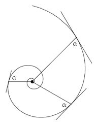Figure 2.3: A logarithmic spiral with a few of its tangents. Click on the picture to go to the constant angle demo-applet.

Another definition, less mathematical, built on the fact that the characteristic angle is constant is the following: let four bugs, called b₁, b₂, b₃ and b₄, be placed in each corner of a square. Each bug is walking with uniform velocity towards the neighboring bug, i.e. b₁ walks towards b₂, b₂ towards b₃, b₃ towards b₄, and b₄ towards b₁. Their respective path is a logarithmic spiral, or more eloquent, an equiangular spiral. In fact, by symmetry, b₁b₂b₃b₄ will always be a square with centre O - the center of the initial square - and each side corresponds to the direction of the velocity vector of each bug. More precisely, [( Ž) || ( b₁b₂)] is the instantaneous velocity vector of b₁ and so on. But this velocity vector is, per definition, the instantaneous tangent to the bug's path - say b₁ - and thus, this tangent forms a constant angle, p/4, with the radius vector [( Ž) || ( Ob₁)] (cf. figure 2.4).

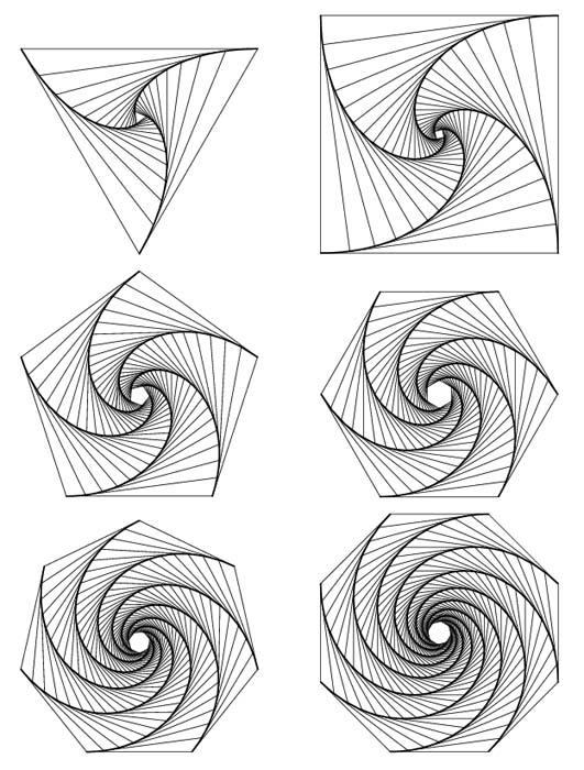
Thus, we have obtained a logarithmic spiral with characteristic angle p/4. Of course, one may consider an arbitrary number n > 2 of bugs walking towards their respective neighbor, and thereby obtain a logarithmic spiral with characteristic angle p(n-2)/(2n) radians, which is half the angle of the polygon corner. This yields some beautiful figures shown on figure 2.5.

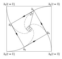Figure 2.4: Four bugs walking towards each other with constant velocity. Click on the image to watch an animation of the bugs displacement.

Figure 2.5: Different configurations of bugs moving towards each other in the way described above.

A third definition is built on Halley's and Nicolas' observations of geometrical progression in the radius vector length. In fact, whereas the archimedean spiral can be seen as a coiled cylinder (for example a rope on a boat deck), the logarithmic spiral can be pictured as a cone coiled upon itself, as D'Arcy Thompson writes in [23], p. 176.

Curves derived from the logarithmic spiral

To any two-dimensional curve, there is associated a series of curves such as the evolute, the envelope, the catacaustic, the pedal or the radial curve, which are obtained by some well-known transformations common to all curves. We will only present four of these here, but there are, of course, many others. A good introduction to such special curves can be found in [16].

The evolute is the locus of centers of the circles of curvature. Roughly speaking, in the two-dimensional case, curvature is the amount by which a curve deviates from a straight line. Correspondingly, the circle of curvature of a curve C, at a given point P, is the best approximation of the curve in a neighborhood of P, and the center O of this circle is, as physicists would say, the instantaneous center of rotation. See also [17] for more details about curvature. The catacaustic is obtained in the following way: consider a light source, projecting rays towards the considered curve. Each ray will of course travel a certain distance d to reach the curve, and thereafter be reflected in it. The locus of the points obtained by proceeding along the reflection in a distance d will form the catacaustic of the curve. The pedal of C is the locus of the intersection points between the perpendicular from a given point O to the tangents of C. The radial curve of C can be constructed as follows: to a point P on C, there corresponds a point Q which is the center of the circle of curvature at P. The radial curve of C with respect to a point O is the locus of the points obtained by translating O of vector QP.

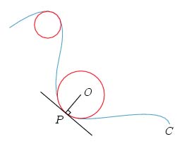Figure 2.7: Circles of curvature.

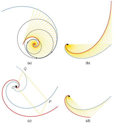
Figure 2.8: The logarithmic spiral (solid blue) and some of its derivatives (solid red): (a) the evolue, some of the circles of curvature and radiis of curvature (yellow lines); (b) the catacaustic, with some rays, originating, in this case, from the pole of the spiral; (c) the radial curve, in this case with respect to the pole, too. For illustrational purpose, the spiral's evolute has also been included (blue dashed line); (d) the pedal, with respect to the pole. Click on the image to go to the "Logarithmic spiral derivatives" applet, where you can expenriment with different curves derived from the logarithmic spiral.

It is interesting to remark that all theses curves, when derived from the logarithmic spiral, are, themselves, spirals of the same class, as depicted on figures 2.8. Of course, some curves might not be spirals at all, such as the negative pedal or the parallel. However, when the derived curve is a logarithmic spiral, it will, always, be one of the same class. The reason can be informally described as follows: all parts of the logarithmic spiral are similar to each other, in the sense that all of these can be mapped onto each other by rotation or scaling - in contradiction to, for instance, the square, where a piece containing a corner is not similar to one containing no corner. A more picturesque description is the following: no matter where you stand on the curve, what is behind you and in front of you is always the same, perhaps just at a different scale, which is also partially due to the fact that the logarithmic spiral is an unending curve at both ends. Therefore, the image of an arbitrary point on the spiral, through one of the mappings used to obtain a derived curve, should be similar to the image of another point on the spiral. Had a derived curve been a logarithmic spiral which was not of the same class, the original curve and the derived one would have an infinity of intersection points, according to Theorem 2.3.1. Thus, there would be one point whose image lies on the original spiral (an intersection point between the two curves), and another point whose image does not lie on it, contradicting our presumption of similarity in the images. Hence, if the derived curve is a logarithmic spiral, it must be of the same class. And this is why Bernoulli talked about the arise of a new curve, for instance the evolute, which is actually similar to the original one.

An unending curve of finite length

Another remarkable property of the logarithmic spiral is that when starting at a point on it, the distance needed to reach the pole, moving along the spiral, is finite, despite that the curve has no endpoint. We will now show that.

Consider a spiral s with polar equation r = a e ^{θ cot α}. To every value of q Î Â corresponds a radius r > 0. Thus, if we stand somewhere on the spiral, we will be able to move inwards or outwards along the curve, infinitely. In this sense, the curve has no end point.

Now, imagine the spiral "rolling out" along a straight line L - the ground one could say - as depicted on figure 2.9. Since P Î s ÇL is the instantaneous rotation centre of O, O being the pole of s, the angle Ð(POQ) is right. Furthermore, a = Ð(OPQ) is constant through the movement, so the pole will move in a fixed direction, perpendicular to OP. Since a < p/2, OQ intersects with the ground, and thus the curve length PQ is given by Pythagores' theorem, namely OP seca.

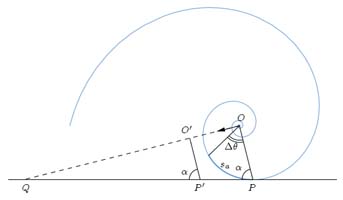Figure 2.9: Spiral rolling along a straight line (without slipping).

This property of an unending curve having finite length is similar the paradox of Achilles and the Tortoise. In this case, we do not divide the real line segment [0,1] into segments of length 1/2, 1/4, 1/8 etc., but divide the spiral into arcs by successive units of angle Dq = 1. If the first piece has length l, the following (moving inwards), will have lengths le^-cota, le^{-2 cota}, etc., as will be shown in the next paragraph. Summing up, the length to the pole is the the limit of the series

l+ le^-cota + le^{-2 cota} + ź

Since a Î ]0,p/ 2[, cota > 0 and hence e^-cota < 1, so the series is convergent, with a well-defined value. From a topological point of view, one can see the pole as a supremum for the set of points that generate the spiral, in the same way that 1 is the supremum for the series ĺ_n=1^Ľ1/2ⁿ used in Achilles' paradox.

Arc length

The above mentioned construction also makes it possible to easily determine the arc length of a logarithmic spiral.

Let s_a be an arc of s delimited by two radiis forming an angle Dq, i.e. an arc of s starting at r(q-Dq) and ending at r(q). We place the spiral such that it touches the ground at r(q). Then we roll it out by an angle Dq, and thus the spiral touches the ground at r(q- Dq). The seeked curve length is therefore the length between the two contact points between the spiral and the ground at r(q) and r(q-Dq). But since OP and O˘P˘ are collinear (forming the same angle a with the ground), and that we know the total distance PQ, a simple application of Thales' theorem gives the arc length:

PQ-PP˘

r(q-Dq)

r(q)

= e^-Dq Ţ PP˘ = (1 - e^-Dq) r(q)seca.

It is funny to mention that if we had used the classical way of finding a curve length using integrals, we would have a lot of trouble since these a very hard, if not impossible, to find. Jacob Bernoulli did that in 1679 and encountered so-called elliptic integrals!

The spiral is a gnomon

In "On Growth and Form" [23], D'Arcy Thompson writes:

"It is characteristic of the growth of the horn, of the shell, and of all other organic forms in which an equiangular spiral can be recognized, that each successive increment of growth is similar, and similarly magnified, and similarly situated to its predecessor, and is in consequence a gnomon to the entire pre-existing structure."

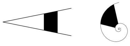
On the right graph of figure 2.15, we have shown the section in question, delimited by two radiis. These radiis are mapped, through T, onto vertical lines in L, creating a trapezium. And such a section is a gnomon to the rest of the triangle. Since the isoceles triangle in L can be considered as a spiral where only rotation has been discarded, is is clear that this trapezium represents a gnomon to the spiral.

Figure 2.15: Mapping between similar shapes (gnomons).

Concluding remarks

With the above described theory of logarithmic spirals as a background, we are ready to move towards more interesting domains in which it come to expression, namely the seashells and the plant patterns.

Continue to the spiral patterns in seashells and horns.