The equations file

If you are new to AUTO you might also be new to Fortran. Therefore, this section will equip you with the necessary basics to get started without having to consult other sources about Fortran first. We would like to note here again that the more recent version AUTO2000 allows you to define your ODEs in C. However, it is useful to know about the Fortran version, because all examples in this package are in Fortran, existing codes of ODEs in Fortran will continue to be around for some while, and a number of users actually prefers Fortran over C. Our description will be on the quite old Fortran 77 standard. Newer versions of Fortran are much more flexible, but these are not yet widely available, in particular, not in open source implementations like the popular g77. Furthermore, the restrictions imposed by the Fortran 77 standard are negligible here. At the end of the day all we have to do is to fill in the body of two subroutines.

The equations file name.f must define all of the Fortran subroutines

Subroutine	:	Defines
FUNC	:	right-hand side of ODE (1),
STPNT	:	an a-priory known initial or seed solution,
BCND	:	boundary conditions,
ICND	:	integral conditions,
FOPT	:	objective function,
PVLS	:	user-defined output.

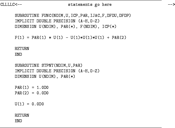
Here, we are only concerned with the first two subroutines, for the others we use default implementations that do nothing. Detailed descriptions of all subroutines, including the empty ones, can be found in the equation files provided with the examples of rauto. Figure 2 shows a sample implementation of the two subroutines FUNC and STPNT. FUNC evaluates the right-hand side of the one-dimensional ODE $\dot{x}=f(x,\lambda,\mu):=\mu + \lambda x - x^3$. The state vector $x$ is in the input array U, the system parameters $(\lambda ,\mu )$ are in the input array PAR, and the vector $f(x,\lambda,\mu)$ is written to the output array F. All other arguments are (normally) unused. STPNT initializes the state variables and parameters with the initial equilibrium solution $x=0$ at $\lambda =1$ and $\mu =0$. The argument NDIM is (normally) unused.

Figure: Sample subroutines FUNC for the ODE $\dot{x}=\mu + \lambda x - x^3$ and STPNT for the starting point $\lambda =1$, $\mu =0$ and $x=0$.

Let us explain step by step the format of the source code in Figure 2. Fortran is not case sensitive, so fortran, Fortran and fORTRAN are all the same. Fortran source code consists of statements and comments. A statement has one or more lines, an initial line and optional continuation lines, which allow splitting of longer statements over several lines. Comments have one or more comment lines. Each type of line has its own format. Initial and continuation lines contain the program statements and consist of four fields, each starting and ending at specific character positions (columns):

Columns	:	Field name
1 through 5	:	statement label,
6	:	continuation indicator,
7 through 72	:	statement,
73 to end of line	:	comment (optional).

Initial lines have an optional statement label, which is a unique number that can be used to refer to it. The continuation indicator is blank and the columns 7 through 72 contain program statements. The statement line can end before column 72, but everything typed from column 73 until the end of line will be treated as a comment, that is, ignored. A continuation line continues a Fortran statement that needs to be split over more than one line. A continuation line has a blank statement label. The continuation indicator contains any Fortran character other than blank or the digit 0. This indicator might be used to count the continuation lines. At least 6 continuation lines must be supported by any Fortran compiler. The statement and comment fields are as for initial lines. A comment line serves solely the purpose of commenting a program and does not affect execution. A comment line is either an entirely blank line or a line beginning with a C, c or an asterisk *. The first line in the source code of Figure 2 is a comment line indicating the fields of initial and continuation lines. All examples that come with rauto contain such comment lines at appropriate locations to make typing easier.

The first statement line `SUBROUTINE ...' defines a subroutine with name FUNC and a list of formal parameters, which are:

Input arguments
NDIM	:	dimension of the ODE (normally unused)
U	:	state or phase-space variables
ICP	:	list of active continuation parameters (normally unused)
PAR	:	system parameters
IJAC	:	Jacobian computation flag (normally unused)
Output arguments
F	:	right-hand side of ODE
DFDU	:	Jacobian (normally unused)
DFDP	:	parameter derivatives (normally unused)

The data type of the formal parameters is not part of the subroutine definition. The body of a subroutine consists of a list of statements that is terminated with an END statement.

The second statement line `IMPLICIT ...' sets the assumed data type for variables beginning with a certain letter to double precision. By default the data type of variables with a name beginning with I, J, K, L, M or N is integer, and the type of all other variables is real (single precision). The data type of variables can also be declared explicitly with a type statement, for example, `DOUBLE PRECISION FOO' declares a variable FOO of type double precision. Type statements inside the body of a subroutine affect the assumed data type of its arguments. Consequently, NDIM, ICP and IJAC are of type integer and U, PAR, F, DFDU and DFDP of type double precision. All computations in AUTO use double precision, so watch out for unwanted conversions. Avoid using single precision functions and constants, because this may lead to poor convergence behavior of AUTO's algorithms. Literal double precision constants are of the form $<$integral-part$>$.$<$fractional-part$>$D[+|-]$<$exponent$>$. Either the integral or the fractional part may be missing. Note the D in the exponential notation, 0.1 and 1.0e-1 are single precision constants. Fortran provides all mathematical standard functions, like trigonometric functions and exponentials. The double precision functions begin with a D, for example, DSIN(X) computes the sine of $x$ in double precision.

The `DIMENSION ...' statement declares a number of arrays. The dimension of an array can be given explicitly in the form [lb:]ub, where lb is the lower and ub the upper bound. If the lower bound is omitted, indexing starts with 1. If an asterisk * is given for the upper bound of the last dimension, the array is a so-called assumed-size array with an unspecified upper bound. However, since Fortran does not check array bounds all declarations in Figure 2 are equivalent. Arrays can be multi-dimensional. Array elements are referenced with round brackets as in U(1).

At the next statement line starts the core part of the subroutine FUNC, namely, the evaluation of the right-hand side of the ODE $\dot{x}=f(x,\lambda,\mu):=\mu + \lambda x - x^3$ at some point $x$. Our ODE is one-dimensional and depends on two parameters, hence, we identify U(1)=$x$, PAR(1)=$\lambda$ and PAR(2)=$\mu$. The statement line `F(1) = ...' evaluates $f(x,\lambda,\mu)$ and assigns the resulting value to the array element F(1). In general, we have U(1)=$x_1$, ..., U(NDIM)=$x_n$ and PAR(1)=$\lambda_1$, ..., PAR(*)=$\lambda_m$ and the components of $f(x,\lambda,\mu)$ are written to F(1),..., F(NDIM). The maximal dimension of an ODE is NDIM=12 by default. This limit can be changed; see [1] for more details. The parameters that can be used in FUNC are PAR(1), ..., PAR(9), parameters PAR(I) with indices I${}\geq 10$ are used internally by AUTO. These internal parameters may be used as continuation parameters or for output purposes. Most commonly, this will be the period of a periodic solution stored in PAR(11) or the rotation number along a locus of Neimark-Sacker points in PAR(12).

The arithmetic expressions that can be used to compute the right-hand side are almost as in other programming languages, just take care of the data types. Fortran provides all mathematical standard functions, the binary arithmetic operators +, -, * and /, the unary sign operators + and -, as well as the exponentiation operator **. The assignment operator is =, multiple assignments as in a=b=c are not allowed.

The body of the subroutine FUNC is terminated with the two consecutive statements RETURN and END. The subroutine STPNT (STarting PoiNT) defined below FUNC initializes U and PAR with an equilibrium point or periodic solution of the ODE at certain parameter values, here $x=0$, $\lambda =1$ and $\mu =0$. It has only one input argument NDIM (normally unused) and two output arguments U and PAR. Note that the initial point must not be a bifurcation point.