In order to perform computations with AUTO you need to set up an equations file and a constants file. The equations file is a Fortran source code file where you specify the right-hand side of your ODE (1) and an initial solution for some parameter values. The equations file offers further functionality, which is explained in the reference manual [1]. The naming convention for the equations file is name.f, where name is a short unique identifier for your problem. The constants file is a plain ASCII text file with name r.name and contains values for certain parameters of AUTO's algorithms as well as some constants of your problem, for example, the dimension of ODE (1). The easiest, most typical, and recommended way to create these two files is to copy an example from this manual or from [1], and to modify the equations and constants file of this copy. There are even commands for this: rdm (rauto) and @dm (AUTO [1]).
After setting up all files we can start computations with AUTO. A single computation with AUTO is called a run. In each run a part of a branch is computed, that is, a part of a parameter dependent family of equilibrium points or periodic solutions. The computation of a complete bifurcation diagram normally consists of multiple runs. We will refer to runs starting at the initial solution specified in the equations file as initial runs. Subsequent runs starting at solutions computed in a previous run will be called restarted runs. There is no difference in the actual computations involved, but the command line of rauto differs slightly for both cases.
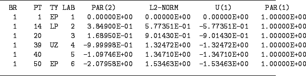
AUTO can perform a stability analysis during continuation. If this feature is enabled AUTO will detect and report a number of so-called special points. Most commonly, these are bifurcation points along a branch at which the solutions change stability. Other special points are points along a branch at which a user defined condition is satisfied. Figure 1 shows a typical output of an AUTO run. The first column BR is the number of the branch, which we will ignore here. Column PT is the number of the solution along the branch, that is, the continuation step in which the solution was computed. Column TY indicates the type of the point. If this column is empty the point is called a regular output point. All other points are special points. For example, LP marks a limit point or saddle-node bifurcation point, and UZ is a point at which the user defined condition PAR(2)![]() is satisfied (within numerical accuracy). Table 1 gives a complete overview over all special point types that AUTO can detect.
is satisfied (within numerical accuracy). Table 1 gives a complete overview over all special point types that AUTO can detect.
|
Column LAB is a unique label that is assigned to any solution that is written to the permanent output of AUTO. These labels are used to identify a restart solution for initializing a restarted run. Often this will be a special point, in which case we perform branch switching to a family of solutions branching off a bifurcation point. For example, at a Hopf bifurcation point HB of an equilibrium point we can switch to the continuation of the periodic solutions emerging from this point.
The first column after LAB is the primary continuation parameter, and the column L2-NORM is the Euclidian norm (equilibrium points) or
![]() norm (periodic solutions) of the solution. The contents of all other columns depends on the actual continuation and will be indicated by an appropriate caption. In Figure 1 these two additional columns are the first coordinate and another free parameter of ODE (1).
norm (periodic solutions) of the solution. The contents of all other columns depends on the actual continuation and will be indicated by an appropriate caption. In Figure 1 these two additional columns are the first coordinate and another free parameter of ODE (1).