Spiral phyllotaxis

Where we use a descriptive model to explain why spirals are observed in the arrangement of seeds in flowers or scales in pinecones; where we explain why the number of visible spirals going in opposite directions are two successive Fibonacci numbers.

Observations in nature

In a daisy or a sunflower, the seeds are not arranged randomly, but are placed along two families of spirals going in opposite directions (called the parastichies), and residing approximately on a disc. The same pattern is observed in pinecones and cactus plants, although the spirals are stretched along three dimensional surfaces.

Figure 4.1: From left to right: A daisy, a sunflower, a pinecone, a cactus. First and fourth pictures kindly lend to us by Pau Atela [3].

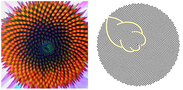
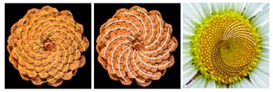
Counting the number of visible spirals in the pinecone and the daisy ,(figure 4.2), we respectively distinguish 8/13 (yellow/white) and 21/34 (black/white) spirals in each directions. These numbers belong to a very curious sequence called the Fibonacci sequence, 0, 1, 1, 2, 3, 5, 8, 13, 21, ź, where each element is the sum of the previous. It is the aim of this chapter to explain the reason for these very specific patterns.

Figure 4.2: Presence of spiral patterns in the scales of the pinecone and the seeds of a daisy.

A descriptive model of Phyllotaxis

Introduction with some examples

In general, the patterns observed in plants is called phyllotaxis, from the Greek phyllo (leaf) and taxis (order), and are established already at a very early stage of the plant's development (in the sunflower, for instance, these patterns are observed when its flower head is only 2mm in diameter). At this early stage, one can not talk about seeds or scales, but small cells known as primordia. Among the patterns observed, three can be distinguished: whorled, distichous and spiral, corresponding to different kinds of distribution of botanical units at a region of the stem (called a node). In whorled phylotaxis, two or more units grow at a same node; this is observed in the Archimes Erecta, where three leaves grow at the same node. In spiral phyllotaxis, only one unit grows at a node, and two successive units form a constant angle, the divergence angle, with the tip of the plant shoot (called the apex). 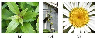Distichous phyllotaxis is a special case of spiral phyllotaxis where this divergence angle is 180^°, and thereby two successive units are formed at opposite sides of the apex. This is depicted, in a three dimensional version, on figure 4.3 (b) (the plant is a Phalaenopsis).

Figure 4.3: Whorled (a), distichous (b) and spiral (c) phyllotaxis. All pictures, again, borrowed from [3].

We will of course study the spiral case exclusively, and refer to [3] for more information on the other patterns.

Descriptive versus explanatory models

In spiral phyllotaxis, there are two models used to explain the observed patterns: the descriptive and the explanatory model. The descriptive one, which we shall study, uses a simplified, geometric approach, with some assumptions such as the value of the divergence angle. However, this model does not care of the dynamical process which the plant, "in reality", undergo, and this has led to a physical model, the explanatory one, which describes the interactions between primordia. In this model, the assumptions are based on hypotheses that Hofmeister [11] formulated in 1868, as a result of a microscopic study of plant shoots:

The newest primordium is formed at the edge of the apex (the apical meristem) which is usually circular, and moves away from it radially.
The period of primordia formation is constant, and is called the plastochrone.
The newest primordium is formed where there is most available space left by the previously formed primordia.

It is the third hypothesis that constitutes the basis for the explanatory model, since it tells that the coordinates of the newest primordium are the ones which minimizes a certain potential energy function. We will not go into more details with this, but complete studies can be found in [12] and [2].

Modelling spiral phyllotaxis

Notations

It is important to realize that we are not interested in a dynamical model which describes evolution of the system of primordia in time, but in a static model, at a given time, where we can analyze the instantaneous position of the N primordia in the system.

In this system, a primordium is identified by its index, that is, its position in the sequence the primordia have been added. Thus, the first primordium added (say, at time t = 0) is denoted p₀, the following p₁ and so on. When we study the spiral patterns, we are only interested in the positions of the primordia, and thus, we assimilate a primordium to a point. And because of the circular movement of the system, it is convenient to consider these points by their polar coordinates, i.e. the position of the i'th primordia is determined by its radius and its angle:

p_i = (q_i, r_i).

If the phytochrome is denoted P, it is not difficult to figure out that the i'th primordia is formed at time t = (N - i) P. Furthermore, assuming that the angle Q between two successive primordia p_i and p_i+1 is constant, or, more generally, that

Dq_n = (

Ž
Op_i

Ž
Op_i+n

) = nQ (2p), n Î N

and that the first primordia has angle q₀ = 0, p_i has angular coordinate q_i = iQ at all time t, in accordance with Hofmeister's first hypothesis of radial movement. Assuming that the velocity of this movement is strictly positive, we get that every primordia lies on distinct circles C, the i'th one lying on circle C_i. Its radius R evolves with time t, i.e. R = R(t) = R((N-i)P). So, all in all, the position of the primordia in the system, at a given time, is

p_i = (i Q, R((N-i)P)), i Î N, i Ł N.

As a consequence, we have to deal with a finite system of primordia, that is, N < Ľ, because otherwise every primordia is infinitely far from the apex O.
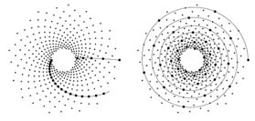
The principle behind the evolution of the system is depicted on figure 4.4 (a).

Figure 4.4: The principle of spiral phyllotaxis. Figure (b) represents the same model as figure (a), but at a later stage, and with a smaller plastochrone. Click on the image to see an animation showing the seeds dispersion in time.

The divergence angle, Q

In most plants, the divergence angle has a very precise value, namely the Golden angle F = 2 p/ f, where f = (1 +Ö5) / 2 is the Golden Ratio. We shall now give an explanation of this phenomenon, starting with the following theorem:

Theorem 5: If Q = [(2 pp)/q], p, q Î Z\{ 0 }, q ł 0, and p/q is an irreducible fraction, then the primordia are aligned along straight lines distributed uniformly on the pencil [0,2p[.

Proof: Since p/q is irreducible, np/q Î Q\\mathbbZČ{ 0 } for all n Î N, n < q, so 2pn p / q (2 p), are different for all n < q. Furthermore, pn Î Z, so it admits a unique representation pn = mq + n˘, where m Î Z, n˘ Î Z, n˘ < q. Thus, 2 p/ q (mq + n˘) (2p) are different for all distinct couples (m, n˘). But 2 p/ q (mq + n˘) (2p) = 2 p m + 2pn˘/q (2p) = 2pn˘ (2p), and thereby 2pn˘ (2p) are all diferent for distinct n˘. Since n˘ < q, 2pp n/q (2p) = 2pn˘/ q Î [0,2p[. Therefore, 2pp n / q divides the interval [0,2p[ into q subintervals of length 2p/q. Moving to the representation in plants, this means that the primordia are aligned along q straight lines, where the angle between two neighboring lines is constant, with value 2p/q. This completes our proof. Now it should come as no surprise that if Q = 2 pa, where a is rational, the packing of the primordia is far from optimal, since we obtain a straight lines configuration (such as the one on figure 4.4 (c), where a = 1 / 5), leaving large gaps in between. One could then think that the solution is simply to use an irrational value of a; in fact, the above mentioned packing will thence not occur, since no two primordium will ever be aligned with the apex. However, the number a = f^-1 is chosen rather that a = p or a = Ö2, although they are all irrational. But, the latter can be quite well approximated by rationals, and therefore, the resulting configuration of the primordium will be very close to the aligned one. So, not only do we want to avoid aligned configurations, we want to get as far as possible away from them. In order to obtain that, we therefore choose the most irrational number, that is, the number which admits the worst rational approximations.

A trivial but important consequence of theorem 4.2.1 is the following:

Lemma 6: If Q = [(2 pp)/q], p, q Î Z\{ 0 }, q ł 0, and p/q is an irreducible fraction, then all the primordia p_i+nq, n Î N such that i+nq < N are aligned along straight lines.
Proof: Simply compute the angle between every q primordia, Dq_q = q Q (2p) = 2 pp (2p) = 0, and the result follows. Now we assume, more generally, that Q = 2pa (2p), where a Î R\{ 0 }. Then we can write Q = 2p(p/q + e), where p / q is a rational approximation to a, and e = a- p / q. Formula becomes:

Dq_q = q Q (2p) = 2pp + 2pq e (2p) = 2 pq e (2p).

In a "sketchy" way, let us join every q primordia p_i+nq, n Î N, n Ł (N-i)/q, starting from one of the points p₀ źp_q-1. When this has been done for all of the starting points, we obviously obtain q curves with no common points. When a has an exact rational approximation, e = 0, so the angle Dq_q between every q primordia is 0. Thereby we rejoin 4.2.2, where the mentioned curves are straight lines. But when a is irrational, i.e. e > 0, the angle between two successive points on the curve is constant and greater than 0. So, for every constant angular increment, we move from a point on C_i to a point on C_i+q.

Try the divergence angle applet, where you can change the value of the divergence angle in real time and see the corresponding configuration of the seeds.

Spiral patterns

We will now investigate on the smooth curve passing through the primordia p_i+nq by claiming the following central theorem, which we might call the fundamental theorem of spiral phyllotaxis:

Theorem 7: If Q = 2pa, where a is irrational and p/q, p, q Î Z\{ 0 }, q > 0 is an irreducible rational approximation to a, and if R(t) is a uniformly increasing function denoting the radius of C_i at time t = (N-i)P, then there exists an affine function f : RŽ R, given by

f(q) = P ć
č N- i + nq
i Q (2p) + nD q_q
q ö
ř ,

such that s Ç C_i+qn = p_i+nq, "n Î N, n Ł (N-i)/q, where s is a curve given in polar coordinates by the equation R(f(q)), q Î R.
In other words, this theorem states that when Q = 2pa where a is irrational, the q curves joining every q primordia, starting from p₀ to p_q-1, are all same spirals (notice that they are not necessarily logarithmic) rotated and scaled properly.

Proof: By definition, p_i+nq Î C_i+nq, so it is sufficient to prove that p_i+nq Î s. As depicted on the picture below, the point p_i+nq has angular coordinate q = i Q(2p) + n Dq_q. From equation , it has radius coordinate R((N-(i+nq))P). What must be proved is therefore that s goes through p_i+nq, i.e. that R(f(q)) = R((N-(i+nq))P) Ű f(q) = (N-(i+nq))P. By the following computation

f(q) = f(i Q(2p) + n Dq_q) = (N - (i+nq))P,

we obtain the desired result. For convenience, we will call the spirals joining every q primordia the "q-spirals".

Now we have proved that when the divergence angle is written as Q = a2p, where a is an irrational number approximated by the fraction irreducible p/q, we can join every q primordia by a spiral. If the quality of the approximation is poor, we will observe very "whorled" spirals. This is due to the fact that e, and thereby Dq_q, is very large. So the angle between two successive primordia that are joined is large. In contrast, as the approximation becomes better, the spirals tend to straight lines, and their number increase since q increases. This is illustrated on figures 4.5, where the divergence angle is Q = 2p/f; the radius function R is the exponential function. Since f is best approximated by the ratio of two successive numbers in the Fibonacci sequence F, we have that the 89-spiral (89 Î F) is almost straight, while the 21-spiral (21 Î F) is more whorled, and the 10-spiral (10 Ď F) does not produce a visible pattern at all.

Figure 4.5: Left: 21- and 89-spirals; right: 10-spiral.

Visible spirals in plants

We shall now explain, informally, the fact that we actually see Fibonacci spirals (or for short, F-spirals) in plants, that is, q-spirals where q Î F. This is not obvious. In fact, in the above, we have demonstrated that non-Fibonacci spirals are more whorled than F-spirals. However, what makes us clearly distinguish some spirals instead of others? What makes us see the 21-spirals of figure 4.5 instead of the 89-spirals? 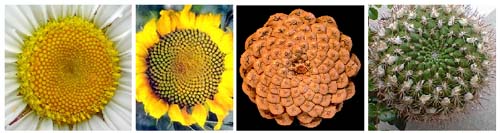Clearly, the quality of the approximation does not affect the visiblilty of the corresponding spiral. For example, look at the pattern observed in plants where the seeds have fixed size, such as the Echinacea purpura below (it will be shown in the next section that the optimal radius function in this case is the square-root function). Try to follow one spiral, say from the apex. You will realize that this becomes more and more difficult as you approach the boundary, since they will be much more whorled. The same holds when starting from a visible spiral on the boundary and moving inwards. This indicates that the number of visible spirals on the boundary of the flower head changes with the number of primordia N in the system.

Figure 4.6: The visible F-spirals in Echinacea purpura are not the same near the apex and near the boundary.

If you look close enough on figure 4.6 (right), you will observe that the spirals are visible when the points which form it are close to each other. More precisely, they are visible when the points on the spirals are successively closest neighbors to one another. So the question is: why is it always a point p_i+n, n Î F, which is the closest neighbor to p_i? In order to answer this, let us consider a q-spiral, where q Î F. Then the angle between two successive points on the spiral is given by Dq_q = 2 pq e(2p), where e is the error associated with the approximation of f. Now let us find another fraction p˘/q˘ which approximates f with the same error e, but where q˘ Ď F. The ratio between two successive numbers of the Fibonacci sequence being the best rational approximation of f, it follows that q˘ > q, and thereby that p_i+q˘ is closer to the apex than p_i+q, since we move inwards as indices icrease. But this is not enough to prove that the q-spirals are more visible than the q˘ ones. We also need to demonstrate that the angle Dq_q is smaller than Dq_q˘. We have not achieved to prove that formally in a general case. However, under the assuption that e is small enough such that Dq_q and Dq_q˘ are smaller that p, we can remove the modulus from their expression, and hence Dq_q < Dq_q˘. Combining the smaller angle Dq_a between two successive primordia on the q-spiral together with the smaller radial distance between these, it follows that p_i+q is closer to p_i than p_i+q˘.

This informal demonstration can be formalized by studying the distance between two primordia p_i and p_i+n,

d(p_i, p_i+n) =

r_i² + r_i+n² - 2r_ir_i+n cosD q_n

by application of the generalized trigonometric formula. Hence, we seek the values of n Î \mathbbN which minimizes the function. We shall support the above demonstration by showing two graphs of this function, evaluated at the discrete points n = 1 ź1000 and n = 1 ź50, respectively, where the radius function is the exponential function. We observe that the minimums are found for n being Fibonacci numbers; from the graph, we deduce that the 21- and 34-spirals are the most visible, while the 13-spiral is only slightly visible.

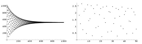Figure 4.7: Plot of the distance function between p₀ and p_n, n Î 1 ź1000 (left) and n Î 1 ź50 (right), with R being the exponential function.

Right- versus left-handed spirals

Now that we have explained that the visible spirals are always F-spirals, it is easy to show that F_n- and F_n+1-spirals are respectively right- and left-handed, that is, they turn inwards and outwards in the counterclockwise direction. In fact, the ratio F_n+1 / F_n approximates the Golden Ratio in an oscillating way, that is

F_n+1

F_n

> f, then

F_n

F_n-1

< f.

Thus, f = F_n+1/F_n + e₁ where e₁ < 0 and f = F_n/F_n-1 + e₂ where e₁ > 0. As a consequence, Dq_{F_n} < 0 while Dq_{F_n-1} > 0, yielding opposite directions in the spirals.

Logarithmic spirals in plants?

Figure 4.6 suggests that the seeds in some plants do not grow once they have been placed. We do not know if this is true, or if the growth rate is so insignificant that the growth can not be observed. And in this case, the observed parastichies are, not surprisingly, no logarithmic spirals, since the phenomenon of growth does not come to expression here. Concerning the packing of the seeds, it would be interesting to show which radius function optimizes it. A straightforward criterion for optimal packing is that the density of the seeds, say d, is the same everywhere on the flower head (i.e. d = constant). This density is the ratio n/A between a given area A and the number of seeds n = at, a constant, inside this area. We are interested in finding the relation between the time t and the linear dimension, which we call l, that is, a function r such that l = r(t). We know that the relation between l and A is given by A = l² = r²(t). Thus we have d = n/A = at/r²(t). In order to obtain the seeked constant density, we must have r(t) = b Öt, b constant. This function can be made equivalent to the radius function R, and, as a consequence of theorem 4.2.3, the observed spirals are square-root spiral with polar equation R(t) linear to Öt.

When the growth rate of the seeds is exponential, in the form r(t) = a₁e^bt, it is obvious that the corresponding radius function is linear to the exponential function, and of the form r(t) = a₂e^bt. If the radius grows at a different rate, even exponentially, either the seeds will collide or the will move away from each other, and thus optimality in the packing clearly does not hold.

Concluding remarks

It was mentioned in [10] that even for exponential growth, the corresponding radius function might not be exponential, and with this function, optimal packings can be obtained. In fact, near the apex, the seeds need to accomodate immediately after they have been emmitted, and little time later, the exponential function governs the radius function completely. So the lack of self-similarity can easily be neglected in the overall plant pattern.

Another phenomenon often observed in the primordia dispersion is the change in phyllotaxis type. In fact, often the first primordia will exhibit distichous phyllotaxis, since there are not enough primordia to make the pattern stable. For instance, when there is only one primordia in the system, it is obvious that the next one will be placed on the opposite side of the apex. The third on will be placed such that the three primordia-configuration will tend to an isoceles triangle, and so on. But this pattern will eventually stabilize, and tends to be of phyllotaxis type spiral.